Utils

utils.density module

Gaussian Mixture Model (GMM) Module for Trajectory Data

This module defines the GaussianMixtureModel class, which fits a Gaussian Mixture Model (GMM) to trajectory data and provides methods to compute density estimates. The class also allows saving and loading the model parameters to/from a file.

The GMM is fitted to time-dependent trajectory data, where each timestep contains a set of data points, and the class allows for computing the GMM-based density at any given timestep for a new input point.

Dependencies:

• jax.numpy: Used for array manipulation and numerical computations.

• sklearn.mixture.GaussianMixture: Used to fit the Gaussian Mixture Model to data.

• pickle: Used for saving and loading model parameters.

• chex: Provides utilities for type and dimensionality checks.

• typing.List, typing.Dict: Used for type hinting.

Class:

• GaussianMixtureModel: Handles the fitting of GMMs to trajectory data, saving/loading the model, and computing the density for a given input.

Class Attributes:

• gms_means: A list storing the means of the Gaussian components for each timestep.

• gms_covs_invs: A list storing the inverses of the covariance matrices for each timestep.

• gms_den: A list of normalization factors for density computation at each timestep.

• gms_weights: A list storing the weights of each Gaussian component for each timestep.

Methods:

• __init__: Initializes the class with empty lists to hold model parameters.

• fit: Fits a GMM to the given trajectory data and stores the relevant parameters (means, inverse covariances, weights).

• to_file: Saves the model parameters to a file using pickle.

• from_file: Loads the model parameters from a file using pickle.

• gmm_density: Computes the density of the GMM at a specified timestep for a given data point.

Example Usage:

from module_name import GaussianMixtureModel
import jax.numpy as jnp

# Initialize the GMM model
gmm = GaussianMixtureModel()

# Example trajectory data (for multiple timesteps)
trajectory = {
    0: jnp.array([[1.0, 2.0], [2.0, 3.0]]),
    1: jnp.array([[1.5, 2.5], [2.5, 3.5]])
}

# Fit the GMM to the trajectory data with 2 components
gmm.fit(trajectory, n_components=2)

# Compute the density at timestep 0 for a new data point
x = jnp.array([1.2, 2.2])
density = gmm.gmm_density(t=0, x=x)

# Save the model to a file
gmm.to_file("gmm_model.pkl")

# Load the model from a file
gmm.from_file("gmm_model.pkl")

class utils.density.GaussianMixtureModel

Bases: object

A class to represent a Gaussian Mixture Model (GMM) that can be fitted to trajectory data and allows for density computation.

gms_means

List to store means of the Gaussian components for each timestep.

Type:

List[jnp.ndarray]

gms_covs_invs

List to store the inverses of the covariance matrices for each timestep.

Type:

List[jnp.ndarray]

gms_den

List to store normalization factors (density denominators) for each timestep.

Type:

List[float]

gms_weights

List to store the weights of each Gaussian component for each timestep.

Type:

List[float]

__init__()

Initializes the GaussianMixtureModel class.

fit(trajectory: dict, n_components: int, seed: int) → None

Fits a Gaussian Mixture Model (GMM) to the given trajectory data.

Parameters:

• trajectory (dict) – A dictionary where each key is a timestep and each value is a 2D array (n_samples, n_features) of data points.

• n_components (int) – The number of clusters (components) to use in the GMM.

• seed (int) – Random seed for reproducibility.

from_file(filename: str)

Loads the GMM model parameters from a file.

Parameters:

filename (str) – The file path to load the model from.

gmm_density(t: int, x: Array) → Array

Computes the GMM density for a given timestep and data point.

Parameters:

• t (int) – The timestep to use for computing the GMM density.

• x (jnp.ndarray) – The data point (array of shape (n_features,)) for which to calculate the density.

Returns:

The computed density value at the specified time and state.

Return type:

jnp.ndarray

to_file(filename: str)

Saves the GMM model parameters to a file.

Parameters:

filename (str) – The file path to save the model to.

utils.features module

Radial Basis Function (RBF) Module

This module provides implementations of various types of radial basis functions (RBFs), which are commonly used in interpolation, machine learning, and numerical approximation.

Radial basis functions take two inputs:

• A data point x (a jax.numpy array).

• A center c (a jax.numpy array).

Each RBF computes a scalar value based on the distance (or other non-linear transformation) between the input x and the center c.

Available Functions:

• rbf_linear: Computes the linear RBF, which is the negative Euclidean distance between x and c.

• rbf_thin_plate_spline: Computes the thin plate spline RBF, which is proportional to the squared distance multiplied by the logarithm of the distance.

• rbf_cubic: Computes the cubic RBF, which sums the cube of differences between x and c.

• rbf_quintic: Computes the quintic RBF, which sums the fifth power of the differences between x and c.

• rbf_multiquadric: Computes the multiquadric RBF, which is the negative square root of the sum of squared differences plus a constant.

• rbf_inverse_multiquadric: Computes the inverse of the multiquadric RBF.

• rbf_inverse_quadratic: Computes the inverse quadratic RBF.

• const: A constant function that always returns 1 regardless of the inputs.

The rbfs dictionary provides a convenient way to access these RBF functions by name.

Usage Example:

To compute an RBF between an input data point and a center, you can use one of the provided RBF functions:

import jax.numpy as jnp
from module_name import rbfs

x = jnp.array([1.0, 2.0])
c = jnp.array([0.5, 1.5])
rbf_value = rbfs['linear'](x, c)

This will compute the linear RBF between x and c.

utils.features.const(x, c)

Computes the constant function.

This function always returns 1, regardless of the input x or the center c.

\[\mathrm{const}(x, c) = 1\]

Parameters:

• x (jnp.ndarray) – Input data point.

• c (jnp.ndarray) – Center (unused).

Returns:

The constant value 1.

Return type:

jnp.ndarray

utils.features.rbf_cubic(x, c)

Computes the cubic radial basis function (RBF).

\[\mathrm{RBF}(x, c) = \sum_{i} (x_i - c_i)^3\]

Parameters:

• x (jnp.ndarray) – Input data point.

• c (jnp.ndarray) – Center of the RBF.

Returns:

The result of the cubic RBF.

Return type:

jnp.ndarray

utils.features.rbf_inverse_multiquadric(x, c)

Computes the inverse multiquadric radial basis function (RBF).

\[\mathrm{RBF}(x, c) = \left( \sqrt{\sum_{i} (x_i - c_i)^2 + 1} \right)^{-1}\]

Parameters:

• x (jnp.ndarray) – Input data point.

• c (jnp.ndarray) – Center of the RBF.

Returns:

The result of the inverse multiquadric RBF.

Return type:

jnp.ndarray

utils.features.rbf_inverse_quadratic(x, c)

Computes the inverse quadratic radial basis function (RBF).

\[\mathrm{RBF}(x, c) = \left(\sum_{i} (x_i - c_i)^2 + 1\right)^{-1}\]

Parameters:

• x (jnp.ndarray) – Input data point.

• c (jnp.ndarray) – Center of the RBF.

Returns:

The result of the inverse quadratic RBF.

Return type:

jnp.ndarray

utils.features.rbf_linear(x, c)

Computes the linear radial basis function (RBF).

This RBF is simply the negative Euclidean distance between the input x and the center c.

\[\mathrm{RBF}(x, c) = -\|x - c\|\]

Parameters:

• x (jnp.ndarray) – Input data point.

• c (jnp.ndarray) – Center of the RBF.

Returns:

The result of the linear RBF.

Return type:

jnp.ndarray

utils.features.rbf_multiquadric(x, c)

Computes the multiquadric radial basis function (RBF).

\[\mathrm{RBF}(x, c) = -\sqrt{\sum_{i} (x_i - c_i)^2 + 1}\]

Parameters:

• x (jnp.ndarray) – Input data point.

• c (jnp.ndarray) – Center of the RBF.

Returns:

The result of the multiquadric RBF.

Return type:

jnp.ndarray

utils.features.rbf_quintic(x, c)

Computes the quintic radial basis function (RBF).

\[\mathrm{RBF}(x, c) = -\sum_{i} (x_i - c_i)^5\]

Parameters:

• x (jnp.ndarray) – Input data point.

• c (jnp.ndarray) – Center of the RBF.

Returns:

The result of the quintic RBF.

Return type:

jnp.ndarray

utils.features.rbf_thin_plate_spline(x, c)

Computes the thin plate spline radial basis function (RBF).

\[\mathrm{RBF}(x, c) = \|x - c\|^2 \log(\|x - c\| + \epsilon)\]

where \(\epsilon\) is a small constant to avoid numerical issues when \(\|x - c\|\) is close to zero.

Parameters:

• x (jnp.ndarray) – Input data point.

• c (jnp.ndarray) – Center of the RBF.

Returns:

The result of the thin plate spline RBF.

Return type:

jnp.ndarray

utils.functions module

This module provides a collection of energy landscape functions commonly used for optimization, testing, and benchmarking purposes. These functions are intentionally not vectorized to enable the use of jax.grad for automatic differentiation. For automatic vectorization, you can use jax.vmap.

The functions in this module represent a variety of optimization landscapes, including convex, non-convex, and complex synthetic functions. They are commonly used in sensitivity analysis, regression tasks, and testing optimization algorithms.

Available Functions:

• styblinski_tang: A non-convex function used to test optimization algorithms.

• holder_table: A complex, non-convex optimization function.

• zigzag_ridge: Another non-convex function, used for benchmarking optimization algorithms.

• oakley_ohagan: A synthetic function used for testing.

• watershed: A complex function that uses an interaction matrix for polynomial expansions.

• ishigami: A function used in sensitivity analysis.

• friedman: A function used in regression and sensitivity analysis.

• sphere: A simple convex function for optimization testing.

• bohachevsky: A non-convex function with trigonometric terms.

• flowers: A non-convex optimization function.

• wavy_plateau: A well-known non-convex function used for optimization testing.

• double_exp: A double exponential function used in optimization problems.

• relu: A rectified linear unit (ReLU) function.

• rotational: A trigonometric-based optimization function.

• flat: A trivial function that returns zero, useful for testing.

Example Usage:

To use any of the provided functions, pass a jax.numpy array as input:

import jax.numpy as jnp
from module_name import potentials_all

v = jnp.array([1.0, 2.0, 3.0])
result = potentials_all['styblinski_tang'](v)

You can also compute the gradient of these functions using jax.grad:

from jax import grad
gradient = grad(potentials_all['styblinski_tang'])(v)

Note:

For vectorized operations, you can use jax.vmap over the provided functions.

utils.functions.bohachevsky(v: Array) → Array

Computes the Bohachevsky function.

\[f(v) = v_1^2 + 2v_2^2 - 0.3 \cos(3 \pi v_1) - 0.4 \cos(4 \pi v_2) + 0.7\]

Parameters:

(jnp.ndarray) (v)

Returns:

jnp.ndarray

Return type:

The result of the Bohachevsky function.

utils.functions.double_exp(v: Array) → Array

Computes the Double Exponential function.

\[f(v) = 200\exp\left(-\frac{||v - m\mathbf{1}||^2}{\sigma}\right) + \exp\left(-\frac{||v + m\mathbf{1}||}{s}\right)\]

where \(d = 3\) and \(s = 20\).

Parameters:

(jnp.ndarray) (v)

Returns:

jnp.ndarray

Return type:

The result of the Double Exponential function.

utils.functions.flat(v: Array) → Array

Computes the Flat function.

Parameters:

(jnp.ndarray) (v)

Returns:

jnp.ndarray

Return type:

The result of the Flat function (always 0).

utils.functions.flowers(v: Array) → Array

Computes the Flowers function.

The function is defined as:

\[f(v) = \sum_{i=1}^{d} \left[ v_i + 2 \cdot \sin(|v_i|^{1.2}) \right]\]

Parameters:

v (jnp.ndarray) – Input array.

Returns:

The result of the Flowers function.

Return type:

jnp.ndarray

utils.functions.friedman(v: Array) → Array

Computes the Friedman function.

\[\begin{split}f(v) = \frac{1}{100}\biggl(10\sin\left(2\pi(z_1 - 7)(z_2 - 7)\right) + 20\left(2(z_1 - 7)\sin(z_2 - 7)- \frac{1}{2}\right)^2 \\\\ + 10\left(2(z_1 - 7)\cos(z_2 - 7) - 1\right)^2 + \frac{1}{10}(z_2 - 7)\sin(2(z_1 - 7))\biggr)\end{split}\]

Parameters:

v (jnp.ndarray) – Input array.

Returns:

The result of the Friedman function, scaled down by a factor of 100.

Return type:

jnp.ndarray

utils.functions.holder_table(v: Array) → Array

Computes the Holder Table function.

\[f(v) = -\left|\sin(v_1)\cos(v_2)\exp\left(\left|1 - \frac{\sqrt{v_1^2 + v_2^2}}{\pi}\right|\right)\right|\]

Parameters:

v (jnp.ndarray) – Input array.

Returns:

The result of the Holder Table function.

Return type:

jnp.ndarray

utils.functions.ishigami(v: Array) → Array

Computes the Ishigami function.

\[f(v) = \sin(z_1) + 7 \sin(z_2)^2 + 0.1 \left(\frac{z_1 + z_2}{2}\right)^4 \sin(z_1)\]

Parameters:

v (jnp.ndarray) – Input array.

Returns:

The result of the Ishigami function.

Return type:

jnp.ndarray

utils.functions.oakley_ohagan(v: Array) → Array

Computes the Oakley-Ohagan function.

Parameters:

v (jnp.ndarray) – Input array.

Returns:

The result of the Oakley-Ohagan function.

\[f(v) = 5 \sum_{i=1}^{d} (\sin(v_i) + \cos(v_i) + v_i^2 + v_i)\]

Return type:

jnp.ndarray

utils.functions.relu(v: Array) → Array

Computes the ReLU (Rectified Linear Unit) function.

\[f(v) = \max(0, v)\]

Parameters:

(jnp.ndarray) (v)

Returns:

jnp.ndarray

Return type:

The result of the ReLU function.

utils.functions.rotational(v: Array) → Array

Computes the Rotational function.

\[f(v) = 10 \cdot \text{ReLU}(\theta + \pi)\]

where \(\theta = \arctan\left(\frac{v_2 + 5}{v_1 + 5}\right)\).

Parameters:

(jnp.ndarray) (v)

Returns:

jnp.ndarray

Return type:

The result of the Rotational function.

utils.functions.sphere(v: Array) → Array

Computes the Sphere function.

\[f(v) = -10||x||^2\]

Parameters:

(jnp.ndarray) (v)

Returns:

jnp.ndarray

Return type:

The result of the Sphere function.

utils.functions.styblinski_tang(v: Array) → Array

Computes the Styblinski-Tang function.

\[f(v) = 0.5 \sum_{i=1}^{d} (v_i^4 - 16v_i^2 + 5v_i)\]

Parameters:

v (jnp.ndarray) – Input array.

Returns:

The result of the Styblinski-Tang function.

Return type:

jnp.ndarray

utils.functions.watershed(v: Array) → Array

Computes the Watershed function.

The function is defined as:

\[f(v) = \frac{1}{10} \sum_{i=1}^{d-1} \left( v_i + v_i^2 \cdot (v_{i+1} + 4) \right)\]

Parameters:

v (jnp.ndarray) – Input array.

Returns:

The result of the Watershed function.

Return type:

jnp.ndarray

utils.functions.wavy_plateau(v: Array) → Array

Computes the Wavy Plateau function.

The function is defined as:

\[f(v) = \sum_{i=1}^{d} \left[\cos(5 \pi v_i) + 0.5 \cdot v_i^4 - 3 \cdot v_i^2 + 1 \right]\]

Parameters:

v (jnp.ndarray) – Input array.

Returns:

The result of the Wavy Plateau function.

Return type:

jnp.ndarray

utils.functions.zigzag_ridge(v: Array) → Array

Computes the Zigzag Ridge function.

\[f(v) = \sum_{i=1}^{d-1} \left[ |v_i - v_{i+1}|^2 + \cos(1.25 \cdot v_i) \cdot (v_i + v_{i+1}) + v_i^2 \cdot v_{i+1} \right]\]

Parameters:

v (jnp.ndarray) – Input array.

Returns:

The result of the Zigzag Ridge function.

Return type:

jnp.ndarray

utils.ot module

This module provides functions for computing Wasserstein distances, Sinkhorn divergences, and optimal transport couplings between two sets of points using the POT (Python Optimal Transport) and JAX-OTT libraries.

Functions

• wasserstein_couplings

  Computes the optimal transport plan (couplings) between two sets of points xs and ys using the POT library.

• wasserstein_loss

  Computes the Wasserstein loss between two sets of points xs and ys, which quantifies the cost of transporting one distribution to match the other.

• sinkhorn_loss

  Computes the Sinkhorn divergence, a regularized Wasserstein distance, between two sets of points xs and ys using the JAX-OTT library.

• compute_couplings

  Computes the couplings between particles in two consecutive batches using the Wasserstein transport plan.

• compute_couplings_sinkhorn

  Computes the Sinkhorn couplings between particles in two consecutive batches using the JAX-OTT library.

• compute_relevant_couplings

  Computes the relevant couplings between particles in two consecutive batches by filtering out the couplings with low weights.

Libraries used

• JAX: A framework for high-performance machine learning and numerical computations with automatic differentiation.

• POT: A Python library for optimal transport calculations.

• JAX-OTT: A library for computing optimal transport using JAX.

• Chex: A library providing assertions and utilities for JAX-related computations.

References

• POT library documentation: https://pythonot.github.io/

• JAX-OTT library documentation: https://ott-jax.readthedocs.io/

utils.ot.compute_couplings(batch: Array, batch_next: Array, time: int) → Array

Computes the couplings between particles in two consecutive batches.

This function uses the wasserstein_couplings function, which leverages the POT (Python Optimal Transport) library to compute the optimal transport plan between two sets of particles.

Parameters:

• batch (jnp.ndarray) – The array of particles at the current timestep with shape (n_particles, n_features).

• batch_next (jnp.ndarray) – The array of particles at the next timestep with shape (n_particles, n_features).

• time (int) – The timestep of batch_next.

Returns:

An array of shape (n_relevant_couplings, 2 * n_features + 2) where each row contains:

• Particle from batch (shape: (n_features,))

• Particle from batch_next (shape: (n_features,))

• Time (float)

• Coupling weight (float)

Only the relevant couplings, where the weight is greater than a threshold, are included.

Return type:

jnp.ndarray

Example

>>> import jax.numpy as jnp
>>> batch = jnp.array([[0., 0.], [1., 0.]])
>>> batch_next = jnp.array([[0., 1.], [2., 2.]])
>>> time = 5
>>> compute_couplings(batch, batch_next, time)
DeviceArray([[0. , 0. , 0. , 1. , 5. , 0.5],
             [1. , 0. , 2. , 2. , 5. , 0.5]], dtype=float32)

References

• POT library documentation: https://pythonot.github.io/

utils.ot.compute_couplings_sinkhorn(batch: Array, batch_next: Array, time: int, epsilon: float = 1.0) → Array

Computes the Sinkhorn couplings (a regularized Wasserstein distance) between two sets of points batch and batch_next.

This function uses the JAX-OTT (Optimal Transport Tools) library to compute the Sinkhorn divergence, which is a regularized version of the Wasserstein distance.

Parameters:

• batch (jnp.ndarray) – The array of particles at the current timestep with shape (n_particles, n_features).

• batch_next (jnp.ndarray) – The array of particles at the next timestep with shape (n_particles, n_features).

• time (int) – The timestep of batch_next.

• epsilon (float, optional) – Regularization parameter for the Sinkhorn algorithm, by default 1.

Returns:

An array of shape (n_relevant_couplings, 2 * n_features + 2) where each row contains:

• Particle from batch (shape: (n_features,))

• Particle from batch_next (shape: (n_features,))

• Time (float)

• Coupling weight (float)

Only the relevant couplings, where the weight is greater than a threshold, are included.

Return type:

jnp.ndarray

utils.ot.compute_relevant_couplings(batch, batch_next, time, weights)

Computes the relevant couplings between particles in two consecutive batches by filtering out the couplings with low weights.

Parameters:

• batch (jnp.ndarray) – The array of particles at the current timestep with shape (n_particles, n_features).

• batch_next (jnp.ndarray) – The array of particles at the next timestep with shape (n_particles, n_features).

• time (int) – The timestep of batch_next.

• weights (jnp.ndarray) – The optimal transport plan matrix of shape (n_samples_x, n_samples_y).

Returns:

An array of shape (n_relevant_couplings, 2 * n_features + 2) where each row contains:

• Particle from batch (shape: (n_features,))

• Particle from batch_next (shape: (n_features,))

• Time (float)

• Coupling weight (float)

Only the relevant couplings, where the weight is greater than a threshold, are included.

Return type:

jnp.ndarray

utils.ot.sinkhorn_loss(xs: Array, ys: Array, epsilon: float = 1.0) → float

Computes the Sinkhorn divergence (a regularized Wasserstein distance) between two sets of points xs and ys.

This function uses the JAX-OTT (Optimal Transport Tools) library to compute the Sinkhorn divergence, which is a regularized version of the Wasserstein distance.

Parameters:

• xs (jnp.ndarray) – An array of shape (n_samples_x, n_features) representing the first set of points.

• ys (jnp.ndarray) – An array of shape (n_samples_y, n_features) representing the second set of points.

• epsilon (float, optional) – Regularization parameter for the Sinkhorn algorithm, by default 1.

Returns:

The Sinkhorn divergence between the two sets of points.

Return type:

float

Example

>>> import jax.numpy as jnp
>>> from ott.geometry import pointcloud
>>> from ott.problems.linear import linear_problem
>>> from ott.solvers.linear import sinkhorn
>>> xs = jnp.array([[0., 0.], [1., 0.]])
>>> ys = jnp.array([[0., 1.], [2., 2.]])
>>> sinkhorn_loss(xs, ys, epsilon=0.1)
DeviceArray(3.0693126, dtype=float32)

References

• JAX-OTT library documentation: https://ott-jax.readthedocs.io/

utils.ot.wasserstein_couplings(xs: Array, ys: Array) → Array

This function uses the POT (Python Optimal Transport) to compute the optimal transport plan (couplings) between two sets of points xs and ys.

Parameters:

• xs (jnp.ndarray) – An array of shape (n_samples_x, n_features) representing the first set of points.

• ys (jnp.ndarray) – An array of shape (n_samples_y, n_features) representing the second set of points.

Returns:

The optimal transport plan matrix of shape (n_samples_x, n_samples_y).

Return type:

jnp.ndarray

References

• POT library documentation: https://pythonot.github.io/

Example

>>> import jax.numpy as jnp
>>> import ot
>>> xs = jnp.array([[0., 0.], [1., 0.]])
>>> ys = jnp.array([[0., 1.], [2., 2.]])
>>> wasserstein_couplings(xs, ys)
DeviceArray([[0.5, 0. ],
             [0. , 0.5]], dtype=float32)

utils.ot.wasserstein_loss(xs: Array, ys: Array, wasserstein_metric: int) → Array

Computes the Wasserstein loss between two sets of points xs and ys.

The Wasserstein loss quantifies the cost of transporting the distribution of points in xs to match the distribution of points in ys. Since the distance is calculated using the ‘sqeuclidean’, it computes the W2 error.

This function uses the POT (Python Optimal Transport) library.

Parameters:

• xs (jnp.ndarray) – An array of shape (n_samples_x, n_features) representing the first set of points.

• ys (jnp.ndarray) – An array of shape (n_samples_y, n_features) representing the second set of points.

Returns:

A scalar representing the Wasserstein loss between the two distributions.

Return type:

jnp.ndarray

Example

>>> import jax.numpy as jnp
>>> import ot
>>> xs = jnp.array([[0., 0.], [1., 0.]])
>>> ys = jnp.array([[0., 1.], [2., 2.]])
>>> wasserstein_loss(xs, ys)
DeviceArray(3.0, dtype=float32)

References

• POT library documentation: https://pythonot.github.io/

utils.plotting module

This module provides a set of plotting utilities for visualizing data and model predictions using matplotlib. The primary functionalities include plotting couplings between particles, generating level curves, visualizing model predictions, creating heatmaps, comparing execution times of models, and plotting loss comparisons across different model parameters.

Functions

• plot_couplings

  Visualizes connections between two sets of points (circles and crosses) with lines whose widths are proportional to the weights.

• domain_from_data

  Computes the domain boundaries for plotting based on the data.

• grid_from_domain

  Generates a grid of points within a specified domain for visualization purposes.

• plot_level_curves

  Plots the level curves of a given function over a specified domain.

• plot_predictions

  Visualizes the predicted and ground truth particle positions for different timesteps.

• colormap_from_config

  Creates a custom colormap from a configuration dictionary.

• plot_heatmap

  Plots a heatmap of values over a 2D grid.

• plot_boxplot_comparison_models

  Creates a boxplot to compare execution times of different models.

• plot_comparison_models

  Compares two sets of model errors, with optional insets for detailed views.

• plot_loss

  Plots the loss values for different models over varying parameter values.

Usage Example

To plot couplings between two sets of points:

>>> import numpy as np
>>> from matplotlib import pyplot as plt
>>> data = np.array([[0., 0., 0., 1., 5., 0.5], [1., 0., 2., 2., 5., 0.5]])
>>> fig, ax = plot_couplings(data)
>>> plt.show()

utils.plotting.domain_from_data(data: ndarray) → Tuple[Tuple[float, float], Tuple[float, float]]

Calculate the domain boundaries from the data for plotting purposes.

Parameters:

data (np.ndarray) – An array where each row contains at least two coordinates (x, y).

Returns:

A tuple containing two tuples:

• The minimum (x_min, y_min) and

• The maximum (x_max, y_max) coordinates, with additional padding.

Return type:

Tuple[Tuple[float, float], Tuple[float, float]]

Example

>>> import numpy as np
>>> data = np.array([[0., 0.], [2., 2.]])
>>> domain_from_data(data)
((-2.0, -2.0), (4.0, 4.0))

utils.plotting.grid_from_domain(domain: Tuple[Tuple[float, float], Tuple[float, float]], n_samples: int = 100) → Tuple[ndarray, ndarray, ndarray]

Create a grid of points within a specified domain.

Parameters:

• domain (Tuple[Tuple[float, float], Tuple[float, float]]) –

  The domain within which to create the grid. It is a tuple containing two tuples:

  • The lower bounds (x_min, y_min) of the domain.

  • The upper bounds (x_max, y_max) of the domain.

• n_samples (int, optional) – The number of samples (grid points) along each axis. Default is 100.

Returns:

• xnp.ndarray

  The x-coordinates of the grid points.

• ynp.ndarray

  The y-coordinates of the grid points.

• gridnp.ndarray

  The grid of points in (x, y) space. If the domain has more than 2 dimensions, extra dimensions are filled with zeros as to project into the other dimensions.

Return type:

Tuple[np.ndarray, np.ndarray, np.ndarray]

Example

>>> import numpy as np
>>> domain = ((-2.0, -2.0), (4.0, 4.0))
>>> x, y, grid = grid_from_domain(domain)
>>> x.shape, y.shape, grid.shape
((100, 100), (100, 100), (10000, 2))

utils.plotting.plot_couplings(data: ndarray) → Tuple[Figure, Axes]

Plots circles at x coordinates, crosses at y coordinates, and connects them with lines whose widths are proportional to weights.

Parameters:

data (np.ndarray) –

An array of shape (n, 6) where each row contains:

• x0, x1 (coordinates of the circle),

• y0, y1 (coordinates of the cross),

• time label

• w (weight for line width).

Returns:

The matplotlib figure and axis objects of the plot.

Return type:

Tuple[plt.Figure, plt.Axes]

Example

>>> import numpy as np
>>> import matplotlib.pyplot as plt
>>> data = np.array([[0. , 0. , 0. , 1. , 5. , 0.5],
...             [1. , 0. , 2. , 2. , 5. , 0.5]])
>>> fig, ax = plot_couplings(data)
>>> plt.show()  # This will display the plot

utils.plotting.plot_level_curves(function: Callable[[ndarray], ndarray], domain: Tuple[Tuple[float, float], Tuple[float, float]], n_samples: int = 100, dimensions: int = 2, save_to: str | None = None) → Figure

Plot level curves of a function over a specified domain.

Parameters:

• function (Callable[[np.ndarray], np.ndarray]) – A function that takes a numpy array of input values and returns a scalar value. The function is expected to be vectorized over the input.

• domain (Tuple[Tuple[float, float], Tuple[float, float]]) – The domain over which to plot the function. It is a tuple containing: - The lower bounds (x_min, y_min) of the domain. - The upper bounds (x_max, y_max) of the domain.

• n_samples (int, optional) – The number of samples (grid points) along each axis. Default is 100.

• dimensions (int, optional) – The number of dimensions of the function output. Default is 2.

• save_to (Optional[str], default=None) – Directory path where plots should be saved. If None, no plots will be saved.

Returns:

The matplotlib figure object containing the plot.

Return type:

plt.Figure

Example

Here is an example of how to use plot_level_curves to visualize the Styblinski-Tang function:

import jax.numpy as jnp

# Define the Styblinski-Tang function
def styblinski_tang(v: jnp.ndarray) -> jnp.ndarray:
    u = jnp.square(v)
    return 0.5 * jnp.sum(jnp.square(u) - 16 * u + 5 * v)

# Define the domain for plotting
domain = ((-4.0, -4.0), (4.0, 4.0))

# Plot and save the level curves
fig = plot_level_curves(
    function=styblinski_tang,
    domain=domain,
    n_samples=200
)

# Display the plot
plt.show()

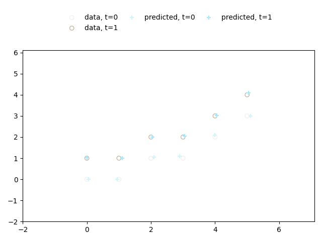
utils.plotting.plot_predictions(predicted: ndarray, data_dict: Dict[int, ndarray], interval: Tuple[int, int] | None, model: str, save_to: str | None = None, n_particles: int = 200) → Figure

Plot predictions and ground truth data for each timestep.

Parameters:

• predicted (np.ndarray) – An array of shape (num_timesteps, num_particles, num_dimensions) containing the predicted particle positions.

• data_dict (Dict[int, np.ndarray]) – A dictionary mapping timesteps to arrays of shape (num_particles, num_dimensions) containing the ground truth particle positions.

• interval (Optional[Tuple[int, int]]) – A tuple specifying the start and end timesteps to plot. If None, plots all timesteps.

• model (str) – A string specifying the model type used to determine color mapping.

• save_to (Optional[str], default=None) – Directory path where plots should be saved. If None, no plots will be saved.

• n_particles (int) – The number of particles to consider for each timestep. Default is 200. If there are less particles either in predictions or in ground truth, that will be the number of particles plotted.

Returns:

The matplotlib figure object containing the plot.

Return type:

plt.Figure

Example

import numpy as np
import matplotlib.pyplot as plt

# Define the ground truth particle positions
data_dict = {
    0: np.array([
        [0., 0.],  [1., 0.],  [2., 1.],  [3., 1.],  [4., 2.],  [5., 3.]]),  # Ground truth at t=0
    1: np.array([
        [0., 1.],  [1., 1.],  [2., 2.],  [3., 2.],  [4., 3.],  [5., 4.]])   # Ground truth at t=1
}

# Define the predicted particle positions
predicted = np.array([
    [[0.05, 0.0], [0.95, 0.0], [2.1, 1.05], [2.9, 1.1], [4.0, 2.1], [5.1, 3.0]],  # Predicted positions at t=0
    [[0.0, 1.02], [1.1, 1.0], [2.05, 2.0], [3.05, 2.05], [4.05, 3.02], [5.05, 4.1]]  # Predicted positions at t=1
])

# Call the function to plot the predictions and ground truth
fig = plot_predictions(predicted=predicted,
                       data_dict=data_dict,
                       interval=(0, 1),
                       model='jkonet-star',
                       )

# Display the plot
plt.show()

utils.sde_simulator module

This module provides tools to simulate Stochastic Differential Equations (SDEs) using explicit and implicit schemes. It includes functionality to generate trajectories based on specified models, potentials, internal energies, and interactions. The simulations are performed using JAX, which enables efficient computations and automatic differentiation.

Classes

• SDESimulator

  Simulates SDEs using an explicit scheme, allowing for the application of potential, internal energy, and interaction components. The class supports forward sampling of trajectories based on the initial condition and a JAX random key.

• SDESimulator_implicit_time

  Simulates SDEs using implicit time-stepping methods. This class is designed to handle time-varying potentials and performs fixed-point iterations to account for implicit dynamics. It supports forward sampling similar to SDESimulator.

Functions

• get_SDE_predictions

  A helper function to choose between explicit and implicit SDE simulators based on the model type and return the simulated trajectories.

Usage example

To simulate trajectories using an explicit SDE simulator:

>>> import jax.numpy as jnp
>>> import jax.random as jrandom
>>> key = jrandom.PRNGKey(0)
>>> init_pp = jnp.array([[0.0, 0.0]])
>>> sde_simulator = SDESimulator(dt=0.01, n_timesteps=100, start_timestep=0, potential=False, internal=0.1, interaction=False)
>>> trajectories = sde_simulator.forward_sampling(key, init_pp)
>>> print(trajectories.shape)  # Output: (101, 1, 2)

For implicit time-stepping with a time-dependent potential:

>>> potential_func = lambda x: 0.5 * jnp.sum(jnp.square(x))
>>> implicit_simulator = SDESimulator_implicit_time(dt=0.01, n_timesteps=100, start_timestep=0, potential=potential_func, internal=False, interaction=False)
>>> trajectories = implicit_simulator.forward_sampling(key, init_pp)
>>> print(trajectories.shape)  # Output: (101, 1, 2)

References

• jax: https://github.com/google/jax

• Stochastic Differential Equations (SDE): https://en.wikipedia.org/wiki/Stochastic_differential_equation

class utils.sde_simulator.SDESimulator(dt: float, n_timesteps: int, start_timestep: int, potential: bool | Callable[[Array], Array], internal: bool | Callable[[Array], Array] | float, interaction: bool | Callable[[Array], Array])

Bases: object

Simulator for Stochastic Differential Equations (SDEs) with an explicit scheme.

Parameters:

• dt (float) – The timestep size for the simulation.

• n_timesteps (int) – The number of timesteps to simulate.

• start_timestep (int) – The initial timestep index for the simulation.

• potential (Optional[Callable[[jnp.ndarray, jnp.ndarray]) – If a callable, it should take a JAX array as input and return the potential. If False, no potential is applied.

• internal (Optional[Callable[[jnp.ndarray, jnp.ndarray]) – If a callable, it should take a JAX array as input and return the internal component. If False, no internal component is used.

• interaction (Optional[Callable[[jnp.ndarray, jnp.ndarray]) – If a callable, it should take a JAX array as input and return the interaction component. If False, no interaction is applied.

forward_sampling(key: jax.random.PRNGKey, init: jnp.ndarray) → jnp.ndarray

Performs forward sampling of the SDE from the initial condition init using the provided random key.

class utils.sde_simulator.SDESimulator_implicit_time(dt: float, n_timesteps: int, start_timestep: int, potential: bool | Callable[[Array], Array], internal: bool | Callable[[Array], Array] | float, interaction: bool | Callable[[Array], Array])

Bases: object

Simulator for Stochastic Differential Equations (SDEs) using implicit methods.

Parameters:

• dt (float) – The timestep size for the simulation.

• n_timesteps (int) – The number of timesteps to simulate.

• start_timestep (int) – The initial timestep index for the simulation. In the case that we are working with time-varying potentials the start time of the simulation is necessary.

• potential (Optional[Callable[[jnp.ndarray, jnp.ndarray]) – If a callable, it should take a JAX array and a time array as input and return the potential. If False, no potential is applied.

• internal (Optional[Callable[[jnp.ndarray, jnp.ndarray]) – If a callable, it should take a JAX array as input and return the internal component. If False, no internal component is used.

• interaction (Optional[Callable[[jnp.ndarray, jnp.ndarray]) – If a callable, it should take a JAX array as input and return the interaction component. If False, no interaction is applied.

forward_sampling(key: jax.random.PRNGKey, init: jnp.ndarray) → jnp.ndarray

Performs forward sampling of the SDE from the initial condition init using the provided random key.

utils.sde_simulator.get_SDE_predictions(model: str, dt: float, n_timesteps: int, start_timestep: int, potential: bool | Callable[[Array], Array], internal: bool | Callable[[Array], Array] | float, interaction: bool | Callable[[Array], Array], key: PRNGKey, init_pp: Array) → Array

Get predictions from a Stochastic Differential Equation (SDE) simulator based on the specified model type.

Depending on the model type, it selects the appropriate SDE simulator (SDESimulator or SDESimulator_implicit_time) and performs forward sampling to generate predictions.

Parameters:

• model (str) – The name of the model to use for simulation. If ‘jkonet-star-time-potential’ is specified, SDESimulator_implicit_time is used; otherwise, SDESimulator is used.

• dt (float) – The timestep size for the SDE simulation.

• n_timesteps (int) – The total number of timesteps to simulate.

• start_timestep (int) – The initial timestep index for the simulation.

• potential (Union[bool, Callable[[jnp.ndarray], jnp.ndarray]]) – If True, a potential function is used in the simulation. If a callable is provided, it should accept a JAX array as input and return the potential. If False, no potential is applied.

• internal (Union[bool, Callable[[jnp.ndarray], jnp.ndarray], float]) – If a float, represents the internal energy scale used in the simulation. If a callable is provided, it should accept a JAX array, returning the internal component. If False, no internal component is used.

• interaction (Union[bool, Callable[[jnp.ndarray], jnp.ndarray]]) – If True, an interaction function is used in the simulation. If a callable is provided, it should accept a JAX array as input and return the interaction component. If False, no interaction is applied.

• key (jax.random.PRNGKey) – A JAX random key used for stochastic processes in the SDE simulation.

• init_pp (jnp.ndarray) – The initial state for the simulation, typically a JAX array representing the starting point of the system.

Returns:

An array representing the simulated trajectories of the system, with shape (n_timesteps + 1, …), where the first dimension corresponds to the timesteps and the remaining dimensions correspond to the state variables of the system.

Return type:

jnp.ndarray